45 excel bar graph labels

How to Create a Bar Chart With Labels Above Bars in Excel In the chart, right-click the Series "Dummy" Data Labels and then, on the short-cut menu, click Format Data Labels. 15. In the Format Data Labels pane, under Label Options selected, set the Label Position to Inside End. 16. Next, while the labels are still selected, click on Text Options, and then click on the Textbox icon. 17. How to Make a Bar Chart in Microsoft Excel Jul 10, 2020 · Adding and Editing Axis Labels To add axis labels to your bar chart, select your chart and click the green “Chart Elements” icon (the “+” icon). From the “Chart Elements” menu, enable the “Axis Titles” checkbox. Axis labels should appear for both the x axis (at the bottom) and the y axis (on the left). These will appear as text boxes.

How to Add Axis Labels in Excel Charts - Step-by-Step (2022) How to add axis titles 1. Left-click the Excel chart. 2. Click the plus button in the upper right corner of the chart. 3. Click Axis Titles to put a checkmark in the axis title checkbox. This will display axis titles. 4. Click the added axis title text box to write your axis label.

Excel bar graph labels

how to add data labels into Excel graphs - storytelling with data There are a few different techniques we could use to create labels that look like this. Option 1: The "brute force" technique. The data labels for the two lines are not, technically, "data labels" at all. A text box was added to this graph, and then the numbers and category labels were simply typed in manually. How to add data labels from different column in an Excel chart? Right click the data series in the chart, and select Add Data Labels > Add Data Labels from the context menu to add data labels. 2. Click any data label to select all data labels, and then click the specified data label to select it only in the chart. 3. Add or remove data labels in a chart - support.microsoft.com To label one data point, after clicking the series, click that data point. In the upper right corner, next to the chart, click Add Chart Element > Data Labels. To change the location, click the arrow, and choose an option. If you want to show your data label inside a text bubble shape, click Data Callout.

Excel bar graph labels. How to add total labels to stacked column chart in Excel? Add total labels to stacked column chart in Excel Supposing you have the following table data. 1. Firstly, you can create a stacked column chart by selecting the data that you want to create a chart, and clicking Insert > Column, under 2-D Column to choose the stacked column. See screenshots: And now a stacked column chart has been built. 2. How to Change Excel Chart Data Labels to Custom Values? Go to Formula bar, press = and point to the cell where the data label for that chart data point is defined. Repeat the process for all other data labels, one after another. See the screencast. Points to note: This approach works for one data label at a time. So if you have a large chart, you are in for a lot of clicks and manic mouse maneuvering. How to Insert Axis Labels In An Excel Chart | Excelchat We will go to Chart Design and select Add Chart Element Figure 6 - Insert axis labels in Excel In the drop-down menu, we will click on Axis Titles, and subsequently, select Primary vertical Figure 7 - Edit vertical axis labels in Excel Now, we can enter the name we want for the primary vertical axis label. How to Make a Bar Chart in Excel - Smartsheet 25 Jan 2018 — Data labels show the value associated with the bars in the chart. This information can be useful if the values are close in range. To add data ...

Bar Graph in Excel — All 4 Types Explained Easily To create a simple bar graph, follow these steps: Get your Data ready. Make sure it has one categorical variable and one quantitative secondary variable. In my example from Sheet1, I have the time duration of 6 tasks. Select your Data with headers. Locate and click on the 2-D Clustered Bars option under the Charts group in the Insert Tab. Edit titles or data labels in a chart - support.microsoft.com The first click selects the data labels for the whole data series, and the second click selects the individual data label. Right-click the data label, and then click Format Data Label or Format Data Labels. Click Label Options if it's not selected, and then select the Reset Label Text check box. Top of Page How to Add Total Data Labels to the Excel Stacked Bar Chart For stacked bar charts, Excel 2010 allows you to add data labels only to the individual components of the stacked bar chart. The basic chart function does not allow you to add a total data label that accounts for the sum of the individual components. Fortunately, creating these labels manually is a fairly simply process. How to Create a Bar Chart With Labels Inside Bars in Excel 7. In the chart, right-click the Series "# Footballers" Data Labels and then, on the short-cut menu, click Format Data Labels. 8. In the Format Data Labels pane, under Label Options selected, set the Label Position to Inside End. 9. Next, in the chart, select the Series 2 Data Labels and then set the Label Position to Inside Base.

How do I make excel label every bar in a bar chart? - Super User Here is what I have done: Insert->Pivot Chart Click Clustered Column Right-click on graph, select Format Axis set specify unit interval to 1 Excel now just labels every 2nd bar, even though it would easily fit (I have about 150 bars) with the given label font size. Histogram with Actual Bin Labels Between Bars - Peltier Tech Select the chart, then use Home tab > Paste dropdown > Paste Special to add the copied data as a new series, with category labels in the first column. You don't see the new series, because it's a series of bars with zero height. But you should notice that the wide bars have been squeezed a bit to make room for the added series. How to Combine Two Bar Graphs in Excel (5 Ways) 5 Ways to Combine Two Bar Graphs in Excel. ... Click on the Edit option from the Horizontal Axis Labels group on the right side. After that, you will get the Axis Labels dialog box. Select the range of the year column in the Axis label range box and press OK. Again, ... How to Use Cell Values for Excel Chart Labels Select the chart, choose the "Chart Elements" option, click the "Data Labels" arrow, and then "More Options." Uncheck the "Value" box and check the "Value From Cells" box. Select cells C2:C6 to use for the data label range and then click the "OK" button. The values from these cells are now used for the chart data labels.

Text Labels on a Horizontal Bar Chart in Excel - Peltier Tech Blog

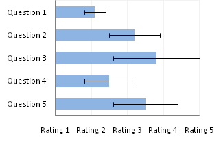
How to label graphs in Excel | Think Outside The Slide If the values are needed, then you will want to use data labels. I suggest placing them inside the end of the column or bar, or just outside the column or bar. This example shows a column graph with data labels only. Example 1 If the message is more related to the ranking of the values, then you can use an axis.

30 How To Label Bar Graph In Excel - Labels Database 2020

How to place labels underneath bar chart - Microsoft Community Answer jpgpinto Replied on February 20, 2012 The names are appearing below the chart axis, that is on value 0.0%. They are on the correct place. If you want them to appear at the bottom of your chart, just select the axis and on the "Format axis" dialog box, on the "Axis options" tab, on the "Axis labels:" option, select "Low". jpgpinto

How can I summarize age ranges and counts in Excel? - Super User

How to Add Total Values to Stacked Bar Chart in Excel Step 4: Add Total Values. Next, right click on the yellow line and click Add Data Labels. Next, double click on any of the labels. In the new panel that appears, check the button next to Above for the Label Position: Next, double click on the yellow line in the chart. In the new panel that appears, check the button next to No line:

How can I hide 0% value in data labels in an Excel Bar Chart - Super User

Excel charts: add title, customize chart axis, legend and data labels Click anywhere within your Excel graph to activate the Chart Tools tabs on the ribbon. On the Layout tab, click Chart Title > Above Chart or Centered Overlay. Link the chart title to some cell on the worksheet For most Excel chart types, the newly created graph is inserted with the default Chart Title placeholder.

How to Create a Bar Chart With Labels Above Bars in Excel

Grouped Bar Chart in Excel - How to Create? (10 Steps) Step 1: Select the chart. With the selection, the Design and Format tabs appear on the Excel ribbon. In the Design tab, choose "change chart type.". Step 2: The "change chart type" window opens, as shown in the following image. Step 3: In the "all charts" tab, click on "bar.".

Quickly Create A Year Over Year Comparison Bar Chart In Excel

How to Make a Bar Graph in Excel: 9 Steps (with Pictures) Add labels for the graph's X- and Y-axes. To do so, click the A1 cell (X-axis) and type in a label, then do the same for the B1 cell (Y-axis). For example, a graph measuring the temperature over a week's worth of days might have "Days" in A1 and "Temperature" in B1. 3 Enter data for the graph's X- and Y-axes.

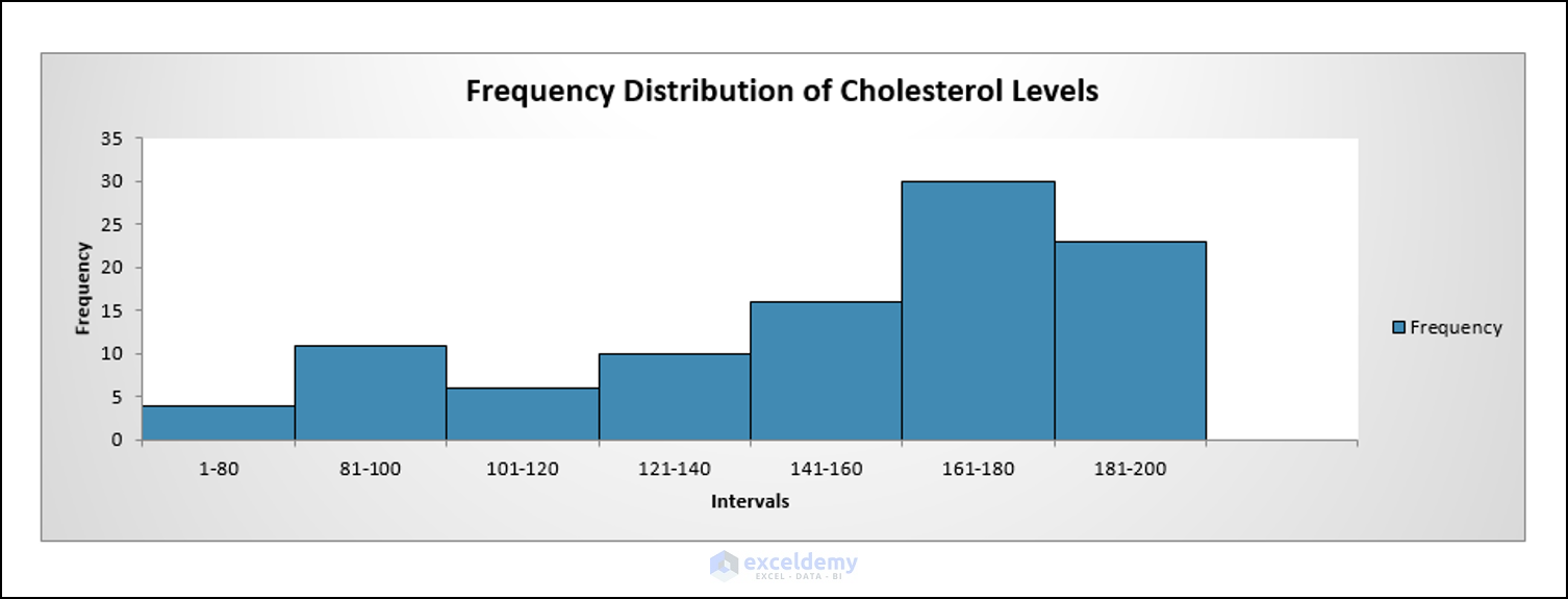
Bar Graph vs Histogram - Difference Between Bar Graph and Histogram!

Bar Chart in Excel | Examples to Create 3 Types of Bar Charts We will add "Data Labels" to the data series in the plotted area. We will click on the chart area to select the data series. Now, as shown in the screenshot, we will right-click on the data series and choose the add data labels to add the data label option. We can move the bar chart to the desired place in the worksheet.

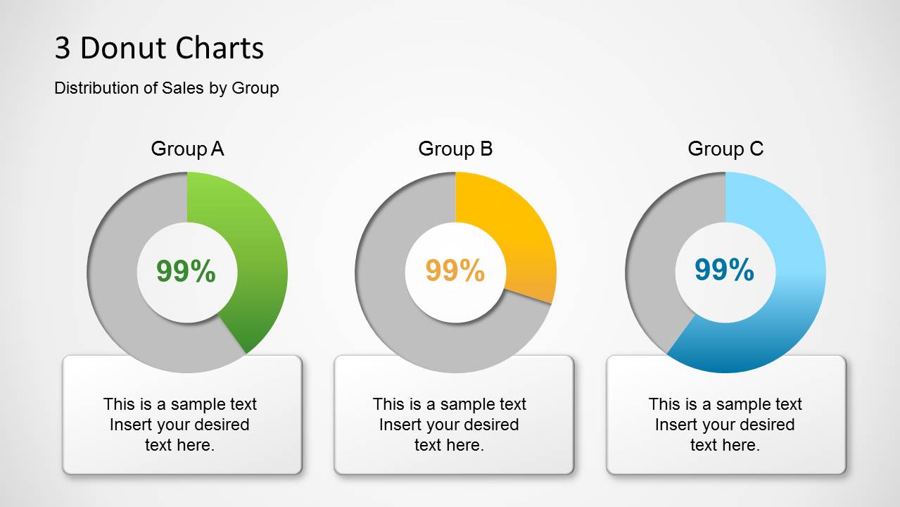
Donut Chart Template for PowerPoint - SlideModel

How to Add Percentages to Excel Bar Chart If we would like to add percentages to our bar chart, we would need to have percentages in the table in the first place. We will create a column right to the column points in which we would divide the points of each player with the total points of all players. We will select range A1:C8 and go to Insert >> Charts >> 2-D Column >> Stacked Column:

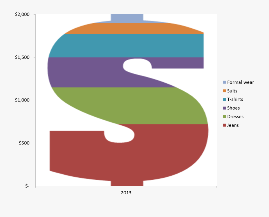
Graph Clipart Secondary Data - Dollar Sign Chart Excel , Free Transparent Clipart - ClipartKey

How to Create Bar Chart in Excel? - EDUCBA Step 1: Select the data > Go to Insert > Bar Chart > Cone Chart. Step 2: Click on the CONE chart, and it will insert the basic chart for you. Step 3: Now, we need to modify the chart by changing its default settings. Remove gridlines of the above Chart. Change the chart title to Sales by month.

How to Create a Bar Chart With Labels Above Bars in Excel

How to Add Two Data Labels in Excel Chart (with Easy Steps) 4 Quick Steps to Add Two Data Labels in Excel Chart. Step 1: Create a Chart to Represent Data. Step 2: Add 1st Data Label in Excel Chart. Step 3: Apply 2nd Data Label in Excel Chart. Step 4: Format Data Labels to Show Two Data Labels. Things to Remember.

How to Create a Bar Chart With Labels Above Bars in Excel

Add or remove data labels in a chart - support.microsoft.com To label one data point, after clicking the series, click that data point. In the upper right corner, next to the chart, click Add Chart Element > Data Labels. To change the location, click the arrow, and choose an option. If you want to show your data label inside a text bubble shape, click Data Callout.

How to label graphs in Excel | Think Outside The Slide

How to add data labels from different column in an Excel chart? Right click the data series in the chart, and select Add Data Labels > Add Data Labels from the context menu to add data labels. 2. Click any data label to select all data labels, and then click the specified data label to select it only in the chart. 3.