44 how to display data labels in excel chart
Create Dynamic Chart Data Labels with Slicers - Excel Campus You basically need to select a label series, then press the Value from Cells button in the Format Data Labels menu. Then select the range that contains the metrics for that series. Click to Enlarge Repeat this step for each series in the chart. If you are using Excel 2010 or earlier the chart will look like the following when you open the file. How to I rotate data labels on a column chart so that they are ... To change the text direction, first of all, please double click on the data label and make sure the data are selected (with a box surrounded like following image). Then on your right panel, the Format Data Labels panel should be opened. Go to Text Options > Text Box > Text direction > Rotate
Adding Data Labels to Your Chart (Microsoft Excel) - ExcelTips (ribbon) Make sure the Design tab of the ribbon is displayed. (This will appear when the chart is selected.) Click the Add Chart Element drop-down list. Select the Data Labels tool. Excel displays a number of options that control where your data labels are positioned. Select the position that best fits where you want your labels to appear.

How to display data labels in excel chart
How to Add Axis Labels in Excel Charts - Step-by-Step (2022) - Spreadsheeto How to add axis titles 1. Left-click the Excel chart. 2. Click the plus button in the upper right corner of the chart. 3. Click Axis Titles to put a checkmark in the axis title checkbox. This will display axis titles. 4. Click the added axis title text box to write your axis label. 5 New Charts to Visually Display Data in Excel 2019 - dummies Aug 26, 2021 · Select the data and labels and then click Insert → Maps → Filled Map. Wait a few seconds for the map to load. Resize and format as desired. For example, you could apply one of the chart styles from the Chart Tools Design tab. To add data labels to the chart, choose Chart Tools Design → Add Chart Element → Data Labels → Show. Pouring ... How to Insert Axis Labels In An Excel Chart | Excelchat We will again click on the chart to turn on the Chart Design tab. We will go to Chart Design and select Add Chart Element. Figure 6 - Insert axis labels in Excel. In the drop-down menu, we will click on Axis Titles, and subsequently, select Primary vertical. Figure 7 - Edit vertical axis labels in Excel. Now, we can enter the name we want ...
How to display data labels in excel chart. Custom Chart Data Labels In Excel With Formulas - How To Excel At Excel Follow the steps below to create the custom data labels. Select the chart label you want to change. In the formula-bar hit = (equals), select the cell reference containing your chart label's data. In this case, the first label is in cell E2. Finally, repeat for all your chart laebls. Excel charts: how to move data labels to legend @Matt_Fischer-Daly . You can't do that, but you can show a data table below the chart instead of data labels: Click anywhere on the chart. On the Design tab of the ribbon (under Chart Tools), in the Chart Layouts group, click Add Chart Element > Data Table > With Legend Keys (or No Legend Keys if you prefer) How to add data labels in excel to graph or chart (Step-by-Step) Add data labels to a chart 1. Select a data series or a graph. After picking the series, click the data point you want to label. 2. Click Add Chart Element Chart Elements button > Data Labels in the upper right corner, close to the chart. 3. Click the arrow and select an option to modify the location. 4. Add or remove data labels in a chart - support.microsoft.com Click the data series or chart. To label one data point, after clicking the series, click that data point. In the upper right corner, next to the chart, click Add Chart Element > Data Labels. To change the location, click the arrow, and choose an option. If you want to show your data label inside a text bubble shape, click Data Callout.
Change the format of data labels in a chart To get there, after adding your data labels, select the data label to format, and then click Chart Elements > Data Labels > More Options. To go to the appropriate area, click one of the four icons ( Fill & Line, Effects, Size & Properties ( Layout & Properties in Outlook or Word), or Label Options) shown here. How to Use Cell Values for Excel Chart Labels - How-To Geek Select the chart, choose the "Chart Elements" option, click the "Data Labels" arrow, and then "More Options." Uncheck the "Value" box and check the "Value From Cells" box. Select cells C2:C6 to use for the data label range and then click the "OK" button. The values from these cells are now used for the chart data labels. How to use data labels in a chart - YouTube Excel charts have a flexible system to display values called "data labels". Data labels are a classic example a "simple" Excel feature with a huge range of o... Add a DATA LABEL to ONE POINT on a chart in Excel All the data points will be highlighted. Click again on the single point that you want to add a data label to. Right-click and select ' Add data label '. This is the key step! Right-click again on the data point itself (not the label) and select ' Format data label '. You can now configure the label as required — select the content of ...
How to Display Percentage in an Excel Graph (3 Methods) Display Percentage in Graph. Select the Helper columns and click on the plus icon. Then go to the More Options via the right arrow beside the Data Labels. Select Chart on the Format Data Labels dialog box. Uncheck the Value option. Check the Value From Cells option. charts - Excel, giving data labels to only the top/bottom X% values ... 1) Create a data set next to your original series column with only the values you want labels for (again, this can be formula driven to only select the top / bottom n values). See column D below. 2) Add this data series to the chart and show the data labels. 3) Set the line color to No Line, so that it does not appear! How to make a Gantt chart in Excel - Ablebits.com 3. Add Duration data to the chart. Now you need to add one more series to your Excel Gantt chart-to-be. Right-click anywhere within the chart area and choose Select Data from the context menu.. The Select Data Source window will open. As you can see in the screenshot below, Start Date is already added under Legend Entries (Series).And you need to add Duration there as well. How to show data label in "percentage" instead of - Microsoft Community Select Format Data Labels Select Number in the left column Select Percentage in the popup options In the Format code field set the number of decimal places required and click Add. (Or if the table data in in percentage format then you can select Link to source.) Click OK Regards, OssieMac Report abuse 8 people found this reply helpful ·
How to Add and Remove Chart Elements in Excel
Excel 2010: Show Data Labels In Chart - AddictiveTips To enable data labels in chart, select the chart and head over to Chart Tools Layout tab, from Labels group, under Data Labels options, select a position. It will show Data labels at specified position. Likewise, from Data Labels pull-down menu, you can change the position of data labels and access other advance options. ← Splash Lite ...

How-to Use Data Labels from a Range in an Excel Chart - Excel ...
Edit titles or data labels in a chart - support.microsoft.com To reposition all data labels for an entire data series, click a data label once to select the data series. To reposition a specific data label, click that data label twice to select it. This displays the Chart Tools , adding the Design , Layout , and Format tabs.

Add data labels and callouts to charts in Excel 365 ...
How to add data labels from different column in an Excel chart? Right click the data series in the chart, and select Add Data Labels > Add Data Labels from the context menu to add data labels. 2. Click any data label to select all data labels, and then click the specified data label to select it only in the chart. 3.

Chart axes, legend, data labels, trendline in Excel - Tech Funda
Showing data labels or values in charts - IBM For a bar, column, line, or area chart, under Series, select the chart type icon.; For a bubble, scatter, Pareto, or progressive chart, click the chart. In the Properties pane, under Chart Labels, double-click the Show Values property.; For bar, column, line, area, Pareto, or progressive charts, to specify the data label format, in the Values list, select what values to display.

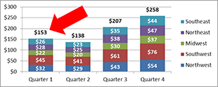
Color Negative Chart Data Labels in Red with downward arrow
How to Change Excel Chart Data Labels to Custom Values? May 05, 2010 · Now, click on any data label. This will select “all” data labels. Now click once again. At this point excel will select only one data label. Go to Formula bar, press = and point to the cell where the data label for that chart data point is defined. Repeat the process for all other data labels, one after another. See the screencast.

Format Number Options for Chart Data Labels in Excel 2011 for Mac
How to Add Data Labels to an Excel 2010 Chart - dummies On the Chart Tools Layout tab, click Data Labels→More Data Label Options. The Format Data Labels dialog box appears. You can use the options on the Label Options, Number, Fill, Border Color, Border Styles, Shadow, Glow and Soft Edges, 3-D Format, and Alignment tabs to customize the appearance and position of the data labels.

How to Use Cell Values for Excel Chart Labels
Display every "n" th data label in graphs - Microsoft Community you can use a free tool created by Rob Bovey, called the XY Chart Labeler. With this tool you can assign a range of cells to be the labels for chart series, instead of the Excel defaults. Using a formula, you can have a text show up in every nth cell and then use that range with the XY Chart Labeler to display as the series label.

excel - How to show series-Legend label name in data labels ...
Excel tutorial: How to use data labels Generally, the easiest way to show data labels to use the chart elements menu. When you check the box, you'll see data labels appear in the chart. If you have more than one data series, you can select a series first, then turn on data labels for that series only. You can even select a single bar, and show just one data label.

How to Add Data Labels to your Excel Chart in Excel 2013
Find, label and highlight a certain data point in Excel scatter graph Select the Data Labels box and choose where to position the label. By default, Excel shows one numeric value for the label, y value in our case. To display both x and y values, right-click the label, click Format Data Labels…, select the X Value and Y value boxes, and set the Separator of your choosing: Label the data point by name

How to Change Excel Chart Data Labels to Custom Values?
Add data labels and callouts to charts in Excel 365 - EasyTweaks.com Step #1: After generating the chart in Excel, right-click anywhere within the chart and select Add labels . Note that you can also select the very handy option of Adding data Callouts.

Change the format of data labels in a chart
How to add and customize chart data labels - Get Digital Help Double press with left mouse button on with left mouse button on a data label series to open the settings pane. Go to tab "Label Options" see image to the right. You have here the option to change the data label position relative to the data point. Center - This places the data label right on the data point.

microsoft excel - Adding data label only to the last value ...
How to Customize Your Excel Pivot Chart Data Labels If you want to label data markers with a category name, select the Category Name check box. To label the data markers with the underlying value, select the Value check box. In Excel 2007 and Excel 2010, the Data Labels command appears on the Layout tab. Also, the More Data Labels Options command displays a dialog box rather than a pane.
Directly Labeling Excel Charts - PolicyViz
Modify Excel Chart Data Range | CustomGuide The new data needs to be in cells adjacent to the existing chart data. Rename a Data Series. Charts are not completely tied to the source data. You can change the name and values of a data series without changing the data in the worksheet. Select the chart; Click the Design tab. Click the Select Data button.

Adding rich data labels to charts in Excel 2013 | Microsoft ...
How to display text labels in the X-axis of scatter chart in ... Actually, there is no way that can display text labels in the X-axis of scatter chart in Excel, but we can create a line chart and make it look like a scatter chart. 1. Select the data you use, and click Insert > Insert Line & Area Chart > Line with Markers to select a line chart. See screenshot: 2. Then right click on the line in the chart to ...

Enable or Disable Excel Data Labels at the click of a button ...
How to add or move data labels in Excel chart? - ExtendOffice 1. Click the chart to show the Chart Elements button . 2. Then click the Chart Elements, and check Data Labels, then you can click the arrow to choose an option about the data labels in the sub menu. See screenshot:

Custom Data Labels with Colors and Symbols in Excel Charts ...
How to Insert Axis Labels In An Excel Chart | Excelchat We will again click on the chart to turn on the Chart Design tab. We will go to Chart Design and select Add Chart Element. Figure 6 - Insert axis labels in Excel. In the drop-down menu, we will click on Axis Titles, and subsequently, select Primary vertical. Figure 7 - Edit vertical axis labels in Excel. Now, we can enter the name we want ...

Add or remove data labels in a chart
5 New Charts to Visually Display Data in Excel 2019 - dummies Aug 26, 2021 · Select the data and labels and then click Insert → Maps → Filled Map. Wait a few seconds for the map to load. Resize and format as desired. For example, you could apply one of the chart styles from the Chart Tools Design tab. To add data labels to the chart, choose Chart Tools Design → Add Chart Element → Data Labels → Show. Pouring ...
![Fixed:] Excel Chart Is Not Showing All Data Labels (2 Solutions)](https://www.exceldemy.com/wp-content/uploads/2022/09/Data-Label-Reference-Excel-Chart-Not-Showing-All-Data-Labels.png)
Fixed:] Excel Chart Is Not Showing All Data Labels (2 Solutions)
How to Add Axis Labels in Excel Charts - Step-by-Step (2022) - Spreadsheeto How to add axis titles 1. Left-click the Excel chart. 2. Click the plus button in the upper right corner of the chart. 3. Click Axis Titles to put a checkmark in the axis title checkbox. This will display axis titles. 4. Click the added axis title text box to write your axis label.

Dynamic Number Format for Millions and Thousands - PK: An ...
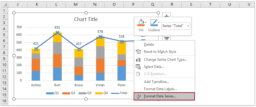
How to add total labels to stacked column chart in Excel?

How to Place Labels Directly Through Your Line Graph in ...

how to add data labels into Excel graphs — storytelling with data
Solved: Area chart data labels not in correct positions ...

Format Data Labels in Excel- Instructions - TeachUcomp, Inc.
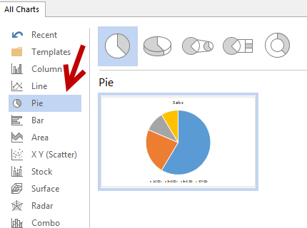
Office: Display Data Labels in a Pie Chart
Excel 2013: Charts
How To Show Or Hide Data Labels On MS Excel? | My Windows Hub

Change the format of data labels in a chart

Add or remove data labels in a chart

Excel Charts: Dynamic Label positioning of line series
How to Add Totals to Stacked Charts for Readability - Excel ...

How To Show Or Hide Data Labels On MS Excel? | My Windows Hub

Format Number Options for Chart Data Labels in PowerPoint ...

Adding rich data labels to charts in Excel 2013 | Microsoft ...

microsoft excel - Adding data label only to the last value ...

Change the format of data labels in a chart

How to Get Colors in Excel Chart Data Lables - Formatting Trick
![Fixed:] Excel Chart Is Not Showing All Data Labels (2 Solutions)](https://www.exceldemy.com/wp-content/uploads/2022/09/Not-Showing-All-Data-Labels-Excel-Chart-Not-Showing-All-Data-Labels.png)
Fixed:] Excel Chart Is Not Showing All Data Labels (2 Solutions)

Directly Labeling Excel Charts - PolicyViz

How can I hide 0% value in data labels in an Excel Bar Chart ...

Display Customized Data Labels on Charts & Graphs

Apply Custom Data Labels to Charted Points - Peltier Tech

Total of chart series – Excel kitchenette

How to add or move data labels in Excel chart?
Post a Comment for "44 how to display data labels in excel chart"